Discrete Fourier Transform#
The discrete Fourier transform (DFT) is a mathematical procedure used to determine the harmonic or frequency content in a discrete time signal sequence. The DFT originates from the continuous Fourier transform, \(X(f)\), defined as follows:
where \(x(t)\) is some continuous time-domain signal.
The DFT is defined as the discrete frequency-domain sequence, \(X(m)\), defined as follows:
where \(x(n)\) is a discrete sequence of time-domain sampled values of the continuous variable \(x(t)\), \(e\) is th base of natural logarithms and \(j=\sqrt{-1}\). The value of \(N\) in the DFT equation determines the following things:
The number of input samples that are needed
The resolution of the frequency-domain results
The amount of processing time necessary to compute an N-point DFT
DFT Concrete Example#
In this concrete DFT example we will let \(N=4\). The rectangular form of this DFT is:
This process is illustrated in more detail in the code below. Feel free to adjust the input to see how the DFT calculation changes.
import numpy as np
import matplotlib.pyplot as plt
# Sample rate and period
Fs = 8e3
Ts = 1/Fs
# Number of samples to use in DFT calculation
N = 8
n = np.arange(0, N)
# Calculate the stop time
t_stop = N * Ts
# Signal parameters
A_1 = 1
f_1 = 1000
theta_1 = 0
A_2 = 0.5
f_2 = 2000
theta_2 = np.pi * 3 / 4
# Discrete signals
x_1 = A_1 * np.sin(2 * np.pi * f_1 * n * Ts + theta_1)
x_2 = A_2 * np.sin(2 * np.pi * f_2 * n * Ts + theta_2)
x_in = x_1 + x_2
# Simulate a continuous signal by setting the sample rate
# sufficiently higher than the discrete sample rate
Fs_cont = 1000 * Fs
Ts_cont = 1/Fs_cont
t_cont = np.arange(0, t_stop, Ts_cont)
# Continuous signals
x_1_cont = A_1 * np.sin(2 * np.pi * f_1 * t_cont + theta_1)
x_2_cont = A_2 * np.sin(2 * np.pi * f_2 * t_cont + theta_2)
x_in_cont = x_1_cont + x_2_cont
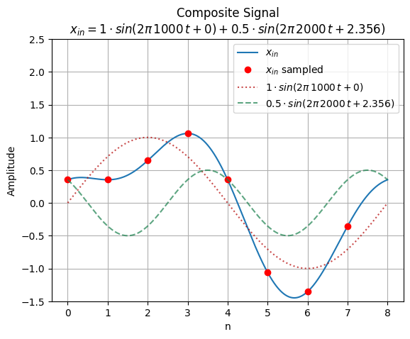
# Plot the composite input data as well as each part of the input data
fig_comp, ax_comp = plt.subplots()
ax_comp.grid()
ax_comp.plot(t_cont/Ts, x_in_cont, label="$x_{in}$")
ax_comp.plot(n, x_in, "ro", label="$x_{in}$ sampled")
ax_comp.plot(t_cont/Ts, x_1_cont, ":", c=(0.7, 0, 0, 0.7),
label=f"${A_1} \cdot sin(2\pi\,{f_1}\,t + {theta_1:.4g})$")
ax_comp.plot(t_cont/Ts, x_2_cont, "--", c=(0.1, 0.5, 0.3, 0.7),
label=f"${A_2} \cdot sin(2\pi\,{f_2}\,t + {theta_2:.4g})$")
# Label and format the plot
ax_comp.set_ylim((-1.5, 2.5))
ax_comp.set_xlabel("n")
ax_comp.set_ylabel("Amplitude")
ax_comp.set_title(f"Composite Signal\n$x_{{in}} = {A_1} \cdot sin(2\pi\,{f_1}\,t + {theta_1:.4g}) + {A_2} \cdot sin(2\pi\,{f_2}\,t + {theta_2:.4g})$")
ax_comp.legend(loc="upper right")
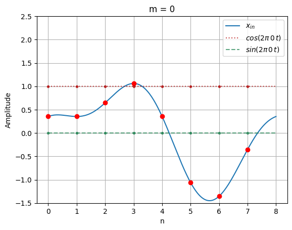
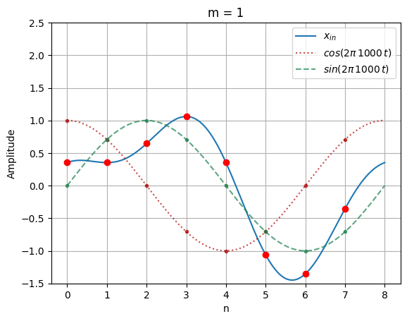
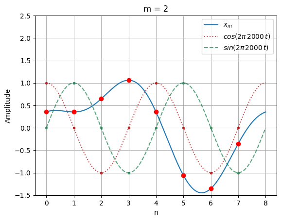
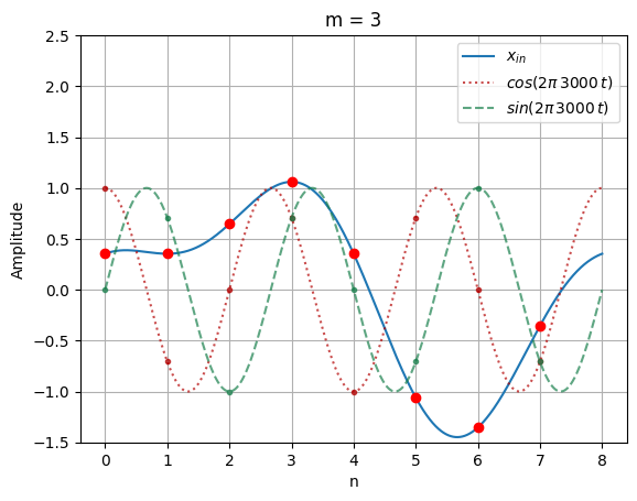
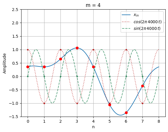
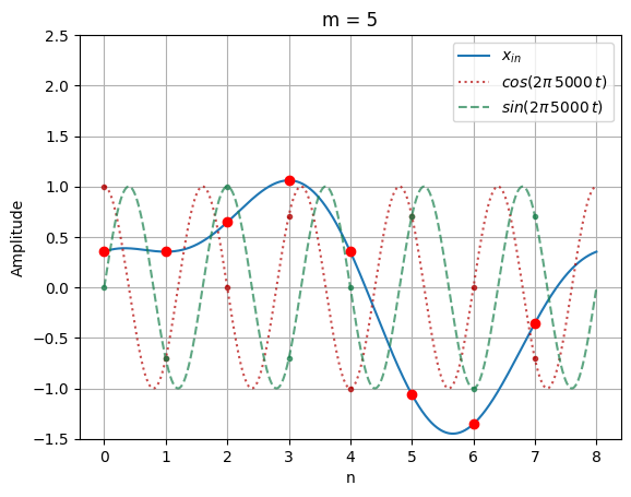
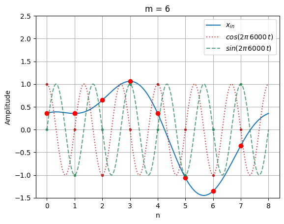
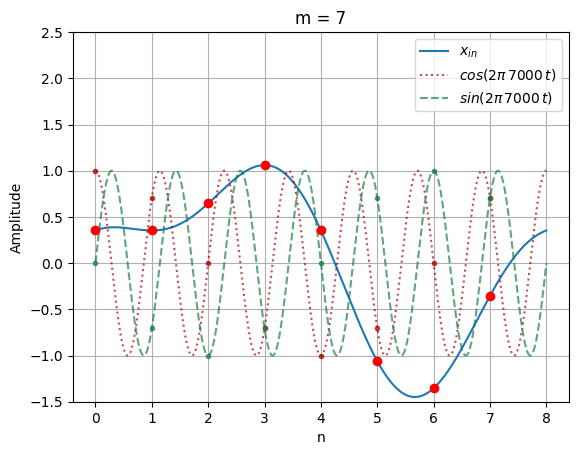
# Create a plot of each complex sinusoid that is used to
# calculate the DFT and perform the DFT calculations
Xm_arr = np.empty(N, dtype=complex)
for m in range(N):
# Generate the complex sinusoids
cos_m = np.cos(2 * np.pi * n * m / N)
sin_m = np.sin(2 * np.pi * n * m / N)
cos_m_cont = np.cos(2 * np.pi * m * Fs / N * t_cont)
sin_m_cont = np.sin(2 * np.pi * m * Fs / N * t_cont)
# Plot the complex sinusoids along with the composite input singal
fig, ax = plt.subplots()
ax.grid()
ax.plot(t_cont/Ts, x_in_cont, label="$x_{in}$")
ax.plot(t_cont/Ts, cos_m_cont, ":", c=(0.7, 0, 0, 0.7),
label=f"$cos(2 \pi \, {round(m*Fs/N, 3):.4g} \,t)$")
ax.plot(t_cont/Ts, sin_m_cont, "--", c=(0.1, 0.5, 0.3, 0.7),
label=f"$sin(2 \pi \, {round(m*Fs/N, 3):.4g} \,t)$")
ax.plot(n, x_in, "ro")
ax.plot(n, cos_m, ".", c=(0.7, 0, 0, 0.7))
ax.plot(n, sin_m, ".", c=(0.1, 0.5, 0.3, 0.7))
# Label and format the plot
ax.set_ylim((-1.5, 2.5))
ax.set_xlabel("n")
ax.set_ylabel("Amplitude")
ax.set_title(f"m = {m}")
ax.legend(loc="upper right")
plt.show()
# Step through each of the DFT calculations
for k in range(N):
real_str = f"({round(x_in[k], 3)} * {round(cos_m[k], 3)})"
imag_str = f"j ({round(x_in[k], 3)} * {round(sin_m[k], 3)})"
if k == 0:
print(f"X({k}) = ", end="")
print(f"{real_str:18}-{imag_str}")
else:
print(f" + {real_str:18}-{imag_str}")
print("\n ........................................................")
for k in range(N):
real_str = f"{round(x_in[k] * cos_m[k], 3)}"
imag_str = f"j {round(x_in[k] * sin_m[k], 3)}"
if k == 0:
print(" = ", end="")
print(f"{real_str:8}-{imag_str}")
else:
print(f" + {real_str:8}-{imag_str}")
print("\n ........................................................")
Xm_real = round(np.sum(x_in * cos_m), 3)
Xm_imag = -round(np.sum(x_in * sin_m), 3)
# Round -0.0 to 0.0 to ensure phase is calculated correctly
if Xm_real == -0.0: Xm_real = 0.0
if Xm_imag == -0.0: Xm_imag = 0.0
print(f" = {Xm_real} - j {Xm_imag}")
print("\n ........................................................")
Xm = complex(Xm_real, Xm_imag)
Xm_arr[m] = Xm
print(f" = {round(np.abs(Xm), 3)} ∠ {round(np.angle(Xm, deg=True), 3)}°")
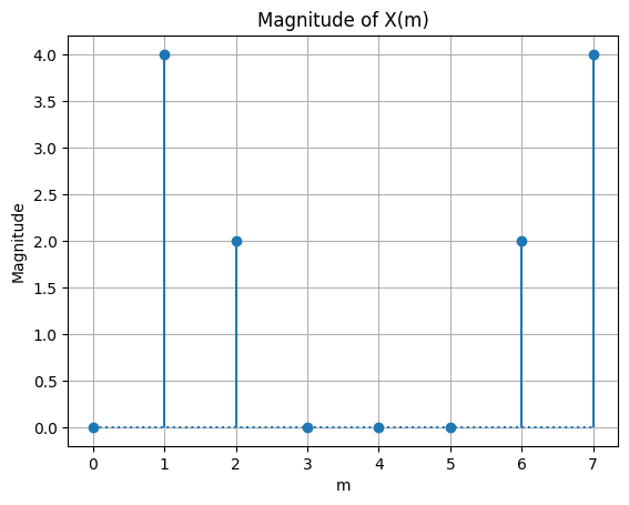
# Plot X(m) magnitude
fig_mag, ax_mag = plt.subplots()
ax_mag.grid()
ax_mag.stem(n, np.abs(Xm_arr), basefmt="C0:")
ax_mag.set_xlabel("m")
ax_mag.set_ylabel("Magnitude")
ax_mag.set_title("Magnitude of X(m)")
# Plot X(m) phase
fig_phase, ax_phase = plt.subplots()
ax_phase.grid()
ax_phase.stem(n, np.angle(Xm_arr, deg=True), basefmt="C0:")
ax_phase.set_xlabel("m")
ax_phase.set_ylabel("Angle (°)")
ax_phase.set_title("Phase of X(m) in degrees")
ax_phase.set_ylim((-180, 180))
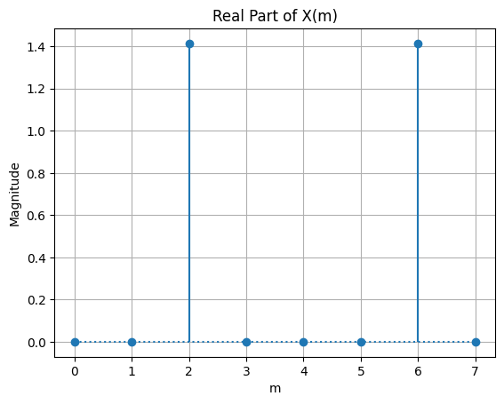
# Plot X(m) real part
fig_real, ax_real = plt.subplots()
ax_real.grid()
ax_real.stem(n, np.real(Xm_arr), basefmt="C0:")
ax_real.set_xlabel("m")
ax_real.set_ylabel("Magnitude")
ax_real.set_title("Real Part of X(m)")
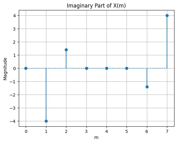
# Plot X(m) imaginary part
fig_imag, ax_imag = plt.subplots()
ax_imag.grid()
ax_imag.stem(n, np.imag(Xm_arr), basefmt="C0:")
ax_imag.set_xlabel("m")
ax_imag.set_ylabel("Magnitude")
ax_imag.set_title("Imaginary Part of X(m)")
pass
X(0) = (0.354 * 1.0)     -j (0.354 * 0.0)
     + (0.354 * 1.0)     -j (0.354 * 0.0)
     + (0.646 * 1.0)     -j (0.646 * 0.0)
     + (1.061 * 1.0)     -j (1.061 * 0.0)
     + (0.354 * 1.0)     -j (0.354 * 0.0)
     + (-1.061 * 1.0)    -j (-1.061 * 0.0)
     + (-1.354 * 1.0)    -j (-1.354 * 0.0)
     + (-0.354 * 1.0)    -j (-0.354 * 0.0)

    ........................................................
     = 0.354   -j 0.0
     + 0.354   -j 0.0
     + 0.646   -j 0.0
     + 1.061   -j 0.0
     + 0.354   -j 0.0
     + -1.061  -j -0.0
     + -1.354  -j -0.0
     + -0.354  -j -0.0

    ........................................................
     = 0.0 - j 0.0

    ........................................................
     = 0.0 ∠ 0.0°
X(0) = (0.354 * 1.0)     -j (0.354 * 0.0)
     + (0.354 * 0.707)   -j (0.354 * 0.707)
     + (0.646 * 0.0)     -j (0.646 * 1.0)
     + (1.061 * -0.707)  -j (1.061 * 0.707)
     + (0.354 * -1.0)    -j (0.354 * 0.0)
     + (-1.061 * -0.707) -j (-1.061 * -0.707)
     + (-1.354 * -0.0)   -j (-1.354 * -1.0)
     + (-0.354 * 0.707)  -j (-0.354 * -0.707)

    ........................................................
     = 0.354   -j 0.0
     + 0.25    -j 0.25
     + 0.0     -j 0.646
     + -0.75   -j 0.75
     + -0.354  -j 0.0
     + 0.75    -j 0.75
     + 0.0     -j 1.354
     + -0.25   -j 0.25

    ........................................................
     = 0.0 - j -4.0

    ........................................................
     = 4.0 ∠ -90.0°
X(0) = (0.354 * 1.0)     -j (0.354 * 0.0)
     + (0.354 * 0.0)     -j (0.354 * 1.0)
     + (0.646 * -1.0)    -j (0.646 * 0.0)
     + (1.061 * -0.0)    -j (1.061 * -1.0)
     + (0.354 * 1.0)     -j (0.354 * -0.0)
     + (-1.061 * 0.0)    -j (-1.061 * 1.0)
     + (-1.354 * -1.0)   -j (-1.354 * 0.0)
     + (-0.354 * -0.0)   -j (-0.354 * -1.0)

    ........................................................
     = 0.354   -j 0.0
     + 0.0     -j 0.354
     + -0.646  -j 0.0
     + -0.0    -j -1.061
     + 0.354   -j -0.0
     + -0.0    -j -1.061
     + 1.354   -j -0.0
     + 0.0     -j 0.354

    ........................................................
     = 1.414 - j 1.414

    ........................................................
     = 2.0 ∠ 45.0°
X(0) = (0.354 * 1.0)     -j (0.354 * 0.0)
     + (0.354 * -0.707)  -j (0.354 * 0.707)
     + (0.646 * -0.0)    -j (0.646 * -1.0)
     + (1.061 * 0.707)   -j (1.061 * 0.707)
     + (0.354 * -1.0)    -j (0.354 * 0.0)
     + (-1.061 * 0.707)  -j (-1.061 * -0.707)
     + (-1.354 * 0.0)    -j (-1.354 * 1.0)
     + (-0.354 * -0.707) -j (-0.354 * -0.707)

    ........................................................
     = 0.354   -j 0.0
     + -0.25   -j 0.25
     + -0.0    -j -0.646
     + 0.75    -j 0.75
     + -0.354  -j 0.0
     + -0.75   -j 0.75
     + -0.0    -j -1.354
     + 0.25    -j 0.25

    ........................................................
     = 0.0 - j 0.0

    ........................................................
     = 0.0 ∠ 0.0°
X(0) = (0.354 * 1.0)     -j (0.354 * 0.0)
     + (0.354 * -1.0)    -j (0.354 * 0.0)
     + (0.646 * 1.0)     -j (0.646 * -0.0)
     + (1.061 * -1.0)    -j (1.061 * 0.0)
     + (0.354 * 1.0)     -j (0.354 * -0.0)
     + (-1.061 * -1.0)   -j (-1.061 * 0.0)
     + (-1.354 * 1.0)    -j (-1.354 * -0.0)
     + (-0.354 * -1.0)   -j (-0.354 * 0.0)

    ........................................................
     = 0.354   -j 0.0
     + -0.354  -j 0.0
     + 0.646   -j -0.0
     + -1.061  -j 0.0
     + 0.354   -j -0.0
     + 1.061   -j -0.0
     + -1.354  -j 0.0
     + 0.354   -j -0.0

    ........................................................
     = 0.0 - j 0.0

    ........................................................
     = 0.0 ∠ 0.0°
X(0) = (0.354 * 1.0)     -j (0.354 * 0.0)
     + (0.354 * -0.707)  -j (0.354 * -0.707)
     + (0.646 * 0.0)     -j (0.646 * 1.0)
     + (1.061 * 0.707)   -j (1.061 * -0.707)
     + (0.354 * -1.0)    -j (0.354 * 0.0)
     + (-1.061 * 0.707)  -j (-1.061 * 0.707)
     + (-1.354 * -0.0)   -j (-1.354 * -1.0)
     + (-0.354 * -0.707) -j (-0.354 * 0.707)

    ........................................................
     = 0.354   -j 0.0
     + -0.25   -j -0.25
     + 0.0     -j 0.646
     + 0.75    -j -0.75
     + -0.354  -j 0.0
     + -0.75   -j -0.75
     + 0.0     -j 1.354
     + 0.25    -j -0.25

    ........................................................
     = 0.0 - j 0.0

    ........................................................
     = 0.0 ∠ 0.0°
X(0) = (0.354 * 1.0)     -j (0.354 * 0.0)
     + (0.354 * -0.0)    -j (0.354 * -1.0)
     + (0.646 * -1.0)    -j (0.646 * 0.0)
     + (1.061 * 0.0)     -j (1.061 * 1.0)
     + (0.354 * 1.0)     -j (0.354 * -0.0)
     + (-1.061 * -0.0)   -j (-1.061 * -1.0)
     + (-1.354 * -1.0)   -j (-1.354 * 0.0)
     + (-0.354 * -0.0)   -j (-0.354 * 1.0)

    ........................................................
     = 0.354   -j 0.0
     + -0.0    -j -0.354
     + -0.646  -j 0.0
     + 0.0     -j 1.061
     + 0.354   -j -0.0
     + 0.0     -j 1.061
     + 1.354   -j -0.0
     + 0.0     -j -0.354

    ........................................................
     = 1.414 - j -1.414

    ........................................................
     = 2.0 ∠ -45.0°
X(0) = (0.354 * 1.0)     -j (0.354 * 0.0)
     + (0.354 * 0.707)   -j (0.354 * -0.707)
     + (0.646 * -0.0)    -j (0.646 * -1.0)
     + (1.061 * -0.707)  -j (1.061 * -0.707)
     + (0.354 * -1.0)    -j (0.354 * 0.0)
     + (-1.061 * -0.707) -j (-1.061 * 0.707)
     + (-1.354 * -0.0)   -j (-1.354 * 1.0)
     + (-0.354 * 0.707)  -j (-0.354 * 0.707)

    ........................................................
     = 0.354   -j 0.0
     + 0.25    -j -0.25
     + -0.0    -j -0.646
     + -0.75   -j -0.75
     + -0.354  -j 0.0
     + 0.75    -j -0.75
     + 0.0     -j -1.354
     + -0.25   -j -0.25

    ........................................................
     = 0.0 - j 4.0

    ........................................................
     = 4.0 ∠ 90.0°
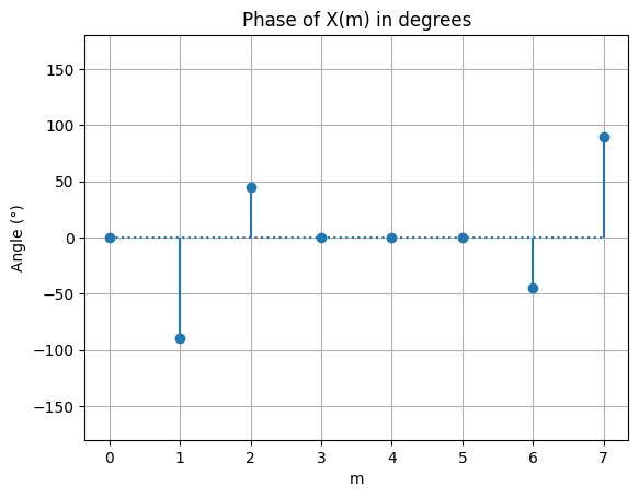
DFT Symmetry#
For a real valued input sequence, the complex DFT outputs will be symmetric about \(m=\frac{N}{2}\). The real parts of the DFT output are even symmetric and the imaginary parts of the DFT output are odd symmetric. This means that the real DFT values on either side of \(m=\frac{N}{2}\) have the same magnitude, but the imaginary DFT values on either side of \(m=\frac{N}{2}\) have their signs flipped. The DFT magnitude is also even symmetric about \(m=\frac{N}{2}\) and the phase is odd symmetric about \(m=\frac{N}{2}\).
DFT Linearity#
The DFT has a property called linearity that states that the DFT of the sum of two signals is equal to the sum of the transforms of each signal. This allows us to take the DFT of signals that contain multiple different frequency components and we will arrive at the same result as if we took the DFT of each individual signal.
DFT Magnitudes#
The DFT output magnitudes are scaled by a factor of \(N\), where \(N\) is the length of the DFT. For a real input signal, the magnitude of the DFT output, \(M_r\), will be equal to:
where \(A_0\) is the amplitude of the real input signal.
For a complex input signal, the magnitude of the DFT output, \(M_c\), will be equal to:
where \(A_0\) is the magnitude of the complex input signal (\(A_0 \, e^{j \, 2 \pi \, f \, n \, T_s}\)).
DFT Frequency Axis#
The frequency that is associated with each value in \(X(m)\) is a function of the sample rate, \(F_s\). The formula to calculate the frequency for a given \(m\) is:
DFT Shifting Theorem#
An important property of the DFT is known as the shifting theorem. This states that a shift in time of a periodic input sequencne manifests itself as a constant phase shift in the angles associated with the DFT results.
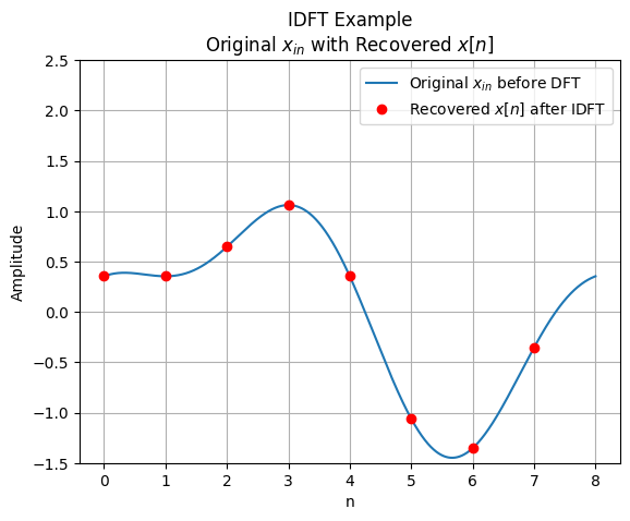
Inverse DFT#
The inverse discrete Fourier transform (IDFT) is a process that allows us to convert frequency-domain data back to the time-domain representation. The IDFT is defined by the following equations:
Notice that the two things that changed between the DFT and the IDFT equations are that:
The IDFT equation has a \(\frac{1}{N}\) scale factor to normalize the gain incurred in the DFT.
The IDFT has the sign flipped in the exponent of the exponential form, and on the imaginary component in the rectangular form.
# Before running this cell, the DFT example code cell above must be run

# Perform the IDFT calculation
xn = np.zeros_like(x_in).astype(np.complex128)
for m in range(N):
    xn += Xm_arr[m] * (np.cos(2 * np.pi * m * n / N) + 1j * np.sin(2 * np.pi * m * n / N))
xn *= 1/N
# Take only the real part of x[n]. The imaginary part cancels out after
# performing the IDFT, and we need x[n] to be real to plot it
xn = np.real(xn)

# Overlay the recovered x[n] with the original input x_in
fig, ax = plt.subplots()
ax.grid()
ax.plot(t_cont/Ts, x_in_cont, label="Original $x_{in}$ before DFT")
ax.plot(n, xn, "ro", label="Recovered $x[n]$ after IDFT")

# Label and format the plot
ax.set_ylim((-1.5, 2.5))
ax.set_xlabel("n")
ax.set_ylabel("Amplitude")
ax.set_title("IDFT Example\nOriginal $x_{in}$ with Recovered $x[n]$")
ax.legend(loc="upper right")
pass