Periodic Sampling

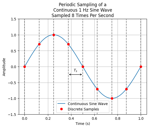
Periodic sampling is the process of representing a continuous signal with a sequence of equally spaced discrete data values. The time between each of the discrete values is known as the sample period, \(T_s\), and the number of discrete values that are sampled in a second is known as the sample rate, \(F_s.\) Illustrated below is a simulated continuous time 1 Hz sine wave that is sampled at a sample rate of 8 Hz.

import numpy as np
import matplotlib.pyplot as plt

# Sinewave frequency
f = 1

# Set the discrete sample rate
Fs_disc = 8
Ts_disc = 1/Fs_disc

# Stop time
t_stop = 1

# Discrete time
t_disc = np.arange(0, t_stop + Ts_disc, Ts_disc)

# Discrete time sine waves
x_1hz_disc = np.sin(2 * np.pi * f * t_disc)

# Set a sample rate that is sufficiently high, such that it appears
# to be continuous for the frequencies we are analyzing
Fs_cont = 1000 * f
Ts_cont = 1/Fs_cont

# Simulated continuous time
t_cont = np.arange(0, t_stop, Ts_cont)

# Simulated continuous time sine waves
x_1hz_cont = np.sin(2 * np.pi * f * t_cont)

# Plot sample time vertical dotted lines
plt.plot(np.concatenate((t_disc, t_disc)).reshape(2, -1),
         np.array(((-2, 2),)*len(t_disc)).T, "--", c=(0, 0, 0, 0.5))

# Plot continuous and discrete sine waves
plt.plot(t_cont, x_1hz_cont, label="Continuous Sine Wave")
plt.plot(t_disc, x_1hz_disc, "ro", label="Discrete Samples")

# Plot sample period arrow
sample_period_bar_idxs = [len(t_disc)//2 - 1, len(t_disc)//2]
x_sample_period_bar = t_disc[sample_period_bar_idxs]
y_sample_period_bar = (min(x_1hz_disc[sample_period_bar_idxs] - 0.25),)*2
plt.annotate("", xy=(x_sample_period_bar[0], y_sample_period_bar[0]),  xycoords="data",
             xytext=(x_sample_period_bar[1],
                     y_sample_period_bar[1]), textcoords="data",
             arrowprops=dict(arrowstyle="<->"))
plt.text(np.mean(x_sample_period_bar),
         y_sample_period_bar[0] + 0.1, "$T_s$", ha="center")

# Label and format plot
plt.xlabel("Time (s)")
plt.ylabel("Amplitude")
plt.title(f"Periodic Sampling of a\nContinuous {f} Hz Sine Wave\nSampled {Fs_disc} Times Per Second")
plt.ylim((-1.5, 1.5))
plt.grid()
plt.legend()
pass