Implementation

Implementation#

In this section, we will cover how to implement linear regression in Python using popular libraries and provide some example use cases to illustrate its practical applications.

Implementing Linear Regression in Python#

Using Scikit-Learn#

Scikit-Learn is a widely used machine learning library in Python that provides a simple and efficient way to implement linear regression.

Installation:
```
pip install scikit-learn
```

Basic Implementation#

import numpy as np
from sklearn.model_selection import train_test_split
from sklearn.linear_model import LinearRegression
from sklearn.metrics import mean_squared_error, r2_score

# Sample data
X = np.array([[0, 0], [1, 1], [2, 2], [3, 3], [4, 4], [5, 5], [6, 6]])
y = np.array([0, 1, 2, 3, 4, 5, 6])

# Split the data into training and testing sets
X_train, X_test, y_train, y_test = train_test_split(X, y, test_size=0.2, random_state=42)

# Create a linear regression model
model = LinearRegression()

# Train the model
model.fit(X_train, y_train)

# Make predictions
y_pred = model.predict(X_test)

# Evaluate the model
mse = mean_squared_error(y_test, y_pred)
r2 = r2_score(y_test, y_pred)

print(f"Mean Squared Error: {mse}")
print(f"R-squared: {r2}")

Mean Squared Error: 0.0
R-squared: 1.0

Custom Implementation#

Implementing linear regression from scratch helps in understanding the underlying mechanics.

import numpy as np

# Sample data
X = np.array([[1], [2], [3], [4], [5]])
y = np.array([1, 2, 3, 4, 5])

# Add a column of ones to include the intercept term
X_b = np.c_[np.ones((X.shape[0], 1)), X]

# Compute the optimal parameters using the Normal Equation
theta_best = np.linalg.inv(X_b.T.dot(X_b)).dot(X_b.T).dot(y)

# Make predictions
X_new = np.array([[1], [2]])
X_new_b = np.c_[np.ones((X_new.shape[0], 1)), X_new]
y_pred = X_new_b.dot(theta_best)

print(f"Predicted values: {y_pred}")

Predicted values: [1. 2.]

Example Use Cases#

Linear regression can be applied to various real-world problems. Here are two example use cases: predicting house prices and forecasting sales.

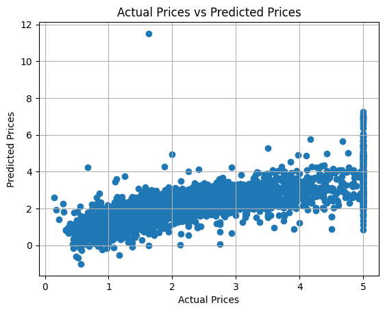
Predicting House Prices#

Predicting house prices is a classic use case for linear regression. By using features such as the size of the house, the number of bedrooms, and location, we can predict the price of a house.

Using the California Housing Dataset#

Load the Dataset:

import numpy as np
from sklearn.datasets import fetch_california_housing
from sklearn.model_selection import train_test_split
from sklearn.linear_model import LinearRegression
from sklearn.metrics import mean_squared_error, r2_score

# Load the California Housing dataset
housing = fetch_california_housing()
X = housing.data
y = housing.target

# Split the data into training and testing sets
X_train, X_test, y_train, y_test = train_test_split(X, y, test_size=0.2, random_state=42)

Create and Train the Model:

# Create a linear regression model
model = LinearRegression()

# Train the model
model.fit(X_train, y_train)

LinearRegression()

In a Jupyter environment, please rerun this cell to show the HTML representation or trust the notebook.
On GitHub, the HTML representation is unable to render, please try loading this page with nbviewer.org.

Make Predictions:

# Make predictions
y_pred = model.predict(X_test)

Evaluate the Model:

# Evaluate the model
mse = mean_squared_error(y_test, y_pred)
r2 = r2_score(y_test, y_pred)

print(f"Mean Squared Error: {mse}")
print(f"R-squared: {r2}")

Mean Squared Error: 0.5558915986952422
R-squared: 0.5757877060324524

Visualize the Results:

import matplotlib.pyplot as plt

# Plot predictions vs actual values
plt.scatter(y_test, y_pred)
plt.xlabel("Actual Prices")
plt.ylabel("Predicted Prices")
plt.title("Actual Prices vs Predicted Prices")
plt.grid()
plt.show()

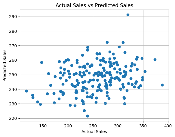
../../../_images/fa29543399db722eadce57d5cebdf343971ce7df3d771b229e230d80fb774bf6.png

Forecasting Sales#

Linear regression can also be used to forecast sales based on historical sales data and other factors such as advertising spend, economic indicators, and seasonal effects.

Using a Custom Dataset#

For this example, let’s generate a simulated sales dataset, sales_data.csv, with advertising, economic_index, seasonality, and sales columns.

Generate a Simulated Dataset:

import pandas as pd
import numpy as np

# Create a sample sales data DataFrame
np.random.seed(42)  # For reproducibility
num_samples = 1000

data = {
    "advertising": np.random.normal(100, 20, num_samples),  # Advertising spend
    "economic_index": np.random.normal(50, 10, num_samples),  # Economic index
    "seasonality": np.random.choice([0, 1], size=num_samples),  # Seasonality (0 or 1)
    "sales": np.random.normal(200, 50, num_samples),  # Sales figures
}

# Introducing some correlation between sales and advertising
data["sales"] += 0.5 * data["advertising"]

# Create DataFrame
sales_data = pd.DataFrame(data)

# Save to CSV
file_path = "sales_data.csv"
sales_data.to_csv(file_path, index=False)

Load the Dataset:

import pandas as pd
from sklearn.model_selection import train_test_split
from sklearn.linear_model import LinearRegression
from sklearn.metrics import mean_squared_error, r2_score

# Load the dataset
data = pd.read_csv("sales_data.csv")
X = data[["advertising", "economic_index", "seasonality"]].values
y = data["sales"].values

# Split the data into training and testing sets
X_train, X_test, y_train, y_test = train_test_split(X, y, test_size=0.2, random_state=42)

Create and Train the Model:

# Create a linear regression model
model = LinearRegression()

# Train the model
model.fit(X_train, y_train)

LinearRegression()