Eigenvalues and Eigenvectors#
Eigenvalues and eigenvectors are fundamental concepts in linear algebra that provide insights into the properties of linear transformations. They are widely used in various machine learning algorithms, particularly in techniques like Principal Component Analysis (PCA). This section will provide a detailed explanation of eigenvalues and eigenvectors, their properties, and their applications in machine learning.
Definition#
Eigenvalues#
An eigenvalue is a scalar that indicates how much the corresponding eigenvector is stretched or compressed during a linear transformation. For a square matrix \(A\), an eigenvalue \(\lambda\) satisfies the equation:
where \(\mathbf{v}\) is the corresponding eigenvector.
Eigenvectors#
An eigenvector is a non-zero vector that remains in the same direction after a linear transformation, though it may be scaled by a corresponding eigenvalue. For a square matrix \(A\), an eigenvector \(\mathbf{v}\) satisfies the equation:
where \(\lambda\) is the corresponding eigenvalue.
Finding Eigenvalues and Eigenvectors#
Characteristic Equation#
To find the eigenvalues of a matrix \(A\), we solve the characteristic equation:
where \(\det\) denotes the determinant of a matrix and \(I\) is the identity matrix of the same dimension as \(A\).
Example#
Consider a 2x2 matrix \(A\):
The characteristic equation is:
Expanding the determinant, we get:
This quadratic equation can be solved for \(\lambda\) to find the eigenvalues.
Finding Eigenvectors#
Once the eigenvalues are determined, we find the corresponding eigenvectors by solving the equation:
for each eigenvalue \(\lambda\).
Example#
For each eigenvalue \(\lambda\), solve:
This yields a system of linear equations, which can be solved to find the eigenvectors.
Properties of Eigenvalues and Eigenvectors#
Sum and Product of Eigenvalues:
The sum of the eigenvalues of a matrix \(A\) is equal to the trace of \(A\) (the sum of the diagonal elements).
The product of the eigenvalues of a matrix \(A\) is equal to the determinant of \(A\).
Diagonalizability:
A matrix \(A\) is diagonalizable if there exists a matrix \(P\) such that \(P^{-1}AP\) is a diagonal matrix. The columns of \(P\) are the eigenvectors of \(A\), and the diagonal elements of \(P^{-1}AP\) are the corresponding eigenvalues.
Applications in Machine Learning#
Principal Component Analysis (PCA)#
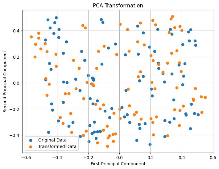
PCA is a dimensionality reduction technique that uses eigenvalues and eigenvectors to transform data into a new coordinate system. The principal components are the eigenvectors of the covariance matrix of the data, and the corresponding eigenvalues represent the variance explained by each principal component.
Compute the Covariance Matrix:
Center the data by subtracting the mean of each feature.
Compute the covariance matrix of the centered data.
Compute Eigenvalues and Eigenvectors:
Find the eigenvalues and eigenvectors of the covariance matrix.
Transform the Data:
Project the data onto the principal components (eigenvectors) to obtain the transformed data.
Example#
import numpy as np
from sklearn.decomposition import PCA
import matplotlib.pyplot as plt

# Generate a synthetic dataset
np.random.seed(42)
X = np.random.rand(100, 2)

# Center the data
X_centered = X - np.mean(X, axis=0)

# Compute the covariance matrix
cov_matrix = np.cov(X_centered, rowvar=False)

# Compute eigenvalues and eigenvectors
eigenvalues, eigenvectors = np.linalg.eig(cov_matrix)

# Sort eigenvectors by eigenvalues in descending order
sorted_indices = np.argsort(eigenvalues)[::-1]
eigenvalues = eigenvalues[sorted_indices]
eigenvectors = eigenvectors[:, sorted_indices]

# Transform the data
X_transformed = np.dot(X_centered, eigenvectors)

# Plot the original and transformed data
plt.figure(figsize=(8, 6))
plt.scatter(X_centered[:, 0], X_centered[:, 1], label="Original Data")
plt.scatter(X_transformed[:, 0], X_transformed[:, 1], label="Transformed Data")
plt.xlabel("First Principal Component")
plt.ylabel("Second Principal Component")
plt.legend()
plt.title("PCA Transformation")
plt.grid()
plt.show()