Descriptive Statistics

Descriptive statistics provide tools for summarizing and describing the main features of a dataset. They are essential for understanding the data’s distribution, central tendency, and variability. These statistics help in making sense of the data and are often the first step in data analysis.

Measures of Central Tendency

Measures of central tendency describe the center or typical value of a dataset. The most common measures are the mean, median, and mode.

Mean

The mean (or average) is the sum of all values divided by the number of values.

\[ \text{Mean} (\mu) = \frac{1}{N} \sum_{i=1}^{N} x_i \]

where \(N\) is the number of observations and \(x_i\) are the individual values.

Median

The median is the middle value of a dataset when the values are sorted in ascending order. If the dataset has an even number of observations, the median is the average of the two middle values.

Mode

The mode is the value that appears most frequently in a dataset. A dataset can have more than one mode if multiple values have the highest frequency.

Measures of Variability

Measures of variability describe the spread or dispersion of a dataset. The most common measures are range, variance, and standard deviation.

Range

The range is the difference between the maximum and minimum values in a dataset.

\[ \text{Range} = \text{Max} - \text{Min} \]

Variance

The variance measures the average squared deviation of each value from the mean.

\[ \text{Variance} (\sigma^2) = \frac{1}{N} \sum_{i=1}^{N} (x_i - \mu)^2 \]

Standard Deviation

The standard deviation is the square root of the variance. It provides a measure of dispersion in the same units as the original data.

\[ \text{Standard Deviation} (\sigma) = \sqrt{\text{Variance}} \]

Graphical Representations

Graphical representations are visual tools for summarizing and exploring data. They help in identifying patterns, trends, and outliers.

Histograms

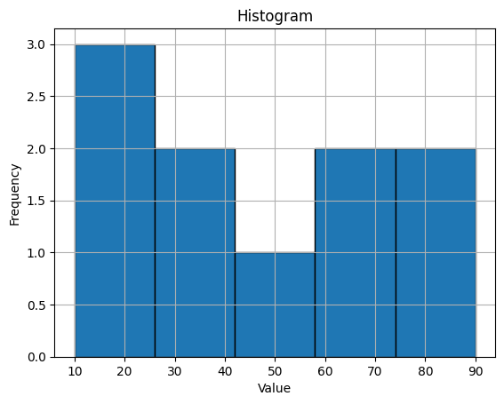
Histograms display the distribution of a dataset by grouping values into bins and plotting the frequency of values in each bin.

Box Plots

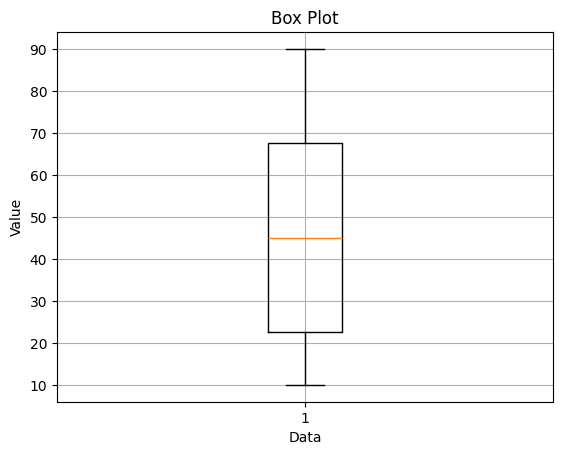
Box plots (or box-and-whisker plots) summarize the distribution of a dataset using the median, quartiles, and outliers.

Scatter Plots

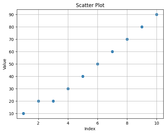
Scatter plots display the relationship between two variables by plotting individual data points on a Cartesian plane.

Examples of Descriptive Statistics in Python

Example 1: Calculating Descriptive Statistics

import numpy as np
from scipy import stats

# Sample data
data = np.array([10, 20, 20, 30, 40, 50, 60, 70, 80, 90])

# Mean
mean = np.mean(data)
print(f"Mean: {mean}")

# Median
median = np.median(data)
print(f"Median: {median}")

# Mode
mode = stats.mode(data)
print(f"Mode: {mode.mode}")

# Range
range_ = np.ptp(data)
print(f"Range: {range_}")

# Variance
variance = np.var(data)
print(f"Variance: {variance}")

# Standard Deviation
std_deviation = np.std(data)
print(f"Standard Deviation: {std_deviation}")

Mean: 47.0
Median: 45.0
Mode: 20
Range: 80
Variance: 681.0
Standard Deviation: 26.095976701399778

Example 2: Plotting Graphical Representations

import matplotlib.pyplot as plt

# Sample data
data = np.array([10, 20, 20, 30, 40, 50, 60, 70, 80, 90])

# Histogram
plt.hist(data, bins=5, edgecolor="black")
plt.xlabel("Value")
plt.ylabel("Frequency")
plt.title("Histogram")
plt.grid()
plt.show()

# Box Plot
plt.boxplot(data)
plt.xlabel("Data")
plt.ylabel("Value")
plt.title("Box Plot")
plt.grid()
plt.show()

# Scatter Plot
x = np.linspace(1, 10, 10)
y = data
plt.scatter(x, y)
plt.xlabel("Index")
plt.ylabel("Value")
plt.title("Scatter Plot")
plt.grid()
plt.show()

Summary

Descriptive statistics provide essential tools for summarizing and describing datasets. They help in understanding the distribution, central tendency, and variability of the data. By mastering these concepts, you can better analyze and interpret data, leading to more informed decisions and insights.

In the next section, we will delve deeper into inferential statistics, which provide methods for making inferences about populations based on sample data.